Please go to Resource page and download it. : )
|
I am glad that I am still working on the project.
We had great discoveries in week 10 that the noise at certain frequencies I mentioned in last report came from the power supply of FPGA. We tried to use a paper box to attenuate the noise from the air, but only to find that the intensity of that certain noise didn’t fall down proportionally as we expected, which means the noise was not from the air. Then we probed the upper board where the microphones are thoroughly to look for the source of this noise. The result shocked us because the noise was from the power. Consider the lower FPGA board provided the power of the upper board, we believed the noise was from FPGA. The further experiments proved our suspect. Actually, the noise was from the power supply of FPGA. After this important discovery, Mr. Richter Ed decided to replace the FPGA board with the more advanced NI Elvis II platform to provide the power of the upper microphone board. And it works! Though we only replace for one out of four boards, the noise was gone and the SNR reached almost the estimated value. With the excitement and the encouragement our new discovery brought to us, we entered week 11. Since all the simulations work as we wish, Mr. Richter asked us to proceed with real world tests. To make the result more accurate, we firstly make a record with a single sound source. The purpose of doing this is to calculate the current lagging timetable, i.e., the current relative positions of 16 microphones. Then we played 2 audios via cellphones from different direction and make records for before-process effect and after-process effect. The comparison results are really encouraging. Though only 16 microphones were involved, we could apparently tell the differences between two records. The beam formed sound from the presumed facing direction was much clearer than the not-beam-formed sound from the same direction under an environment where there was another interfering sound source at a different direction. By now, I could draw a line and encapsulate my project! This might be the last report I wrote for this project although I would like to keep working on this during the coming weeks and months. Good news was that we make big progress during the past period. Since we were stuck somehow, Mr. Richter Ed was intended to search for help from other people. So he asked me to modify the Matlab code as to make it easy to read, understand and test. After week 7, the code was significantly improved. The whole structure was slightly changed for the easiness to read and understand. New scripts and functions were also applied to make the program much smarter and more logical. A script, configuration.m where most of constant and global variables were assigned, was introduced for the consistency and convenience during test. In week 8, a new member Ricky joined my work. He was a senior from Tsinghua University. I am really glad to work with a talent teammate from the top university in China. He suggested using cross correlation in time domain to compute the lag time for each of 64 microphones. His idea did help. This new lag timetable on which shifting is based is dynamic and with high accuracy. The corresponding result is much faster and better. (Pic. 1) Thanks for the improvement we had in week 8, we started over the SNR test in week 9 and found that the terrible performance of SNR might be partly due to the omission of the power of harmonic components of the signal. The main factor of the unexpected SNR, we supposed, was that there were noises at certain frequencies in the background noise. Those noises at certain frequencies were opposite to white Gaussian noise. Their power would be added constructively during beamforming, and leading to higher power gain than expected. Ricky and I had raised the SNR by filtering those noises at certain frequencies (Pic. 2). But there were still several questions we were incapable to answer: 1. Where do the noises come from? 2. Why does the frequency of those noises shift? I was supposed to work on this project for 8 weeks while this was the end of the 9th week. My course process might be over next week, but I will keep working on this project during the rest of my summer vocation, even after new semester begins. I had really struggling time with the project in these two weeks. Since we had already achieved real-time DOA detection before, I was supposed to testify the effectiveness of the beamforming algorithm with real time data. For the convenience of the verification, I recorded a new audio with a 4000Hz sinusoidal signal, naming the file ‘uPhoneArray_LoudSignal.bin’. Assuming that background noise is white Gaussian distributed, beamforming based on a 64-microphone array could theoretically raise SNR by roughly 18dB, which has been proved mathematically and under simulation environment (See Pic. 1). However, the result (See Pic. 2) from real data was so disappointing that Mr. Richter Ed and I got stuck to this problem for two weeks. We recalculated the theoretical improvement on SNR, tested the accuracy of Matlab code function by function, block by block and adjusted the way we computed SNR. Everything seemingly worked correctly except SNR. By the end of the 6th week, we were still not able to pinpoint the conflict. Amplification difference among 64 microphones, non-while-Gaussian-distributed noise, the approach to gain signal and noise power, the DC component in signal and so on may all result in the deviation from theory.  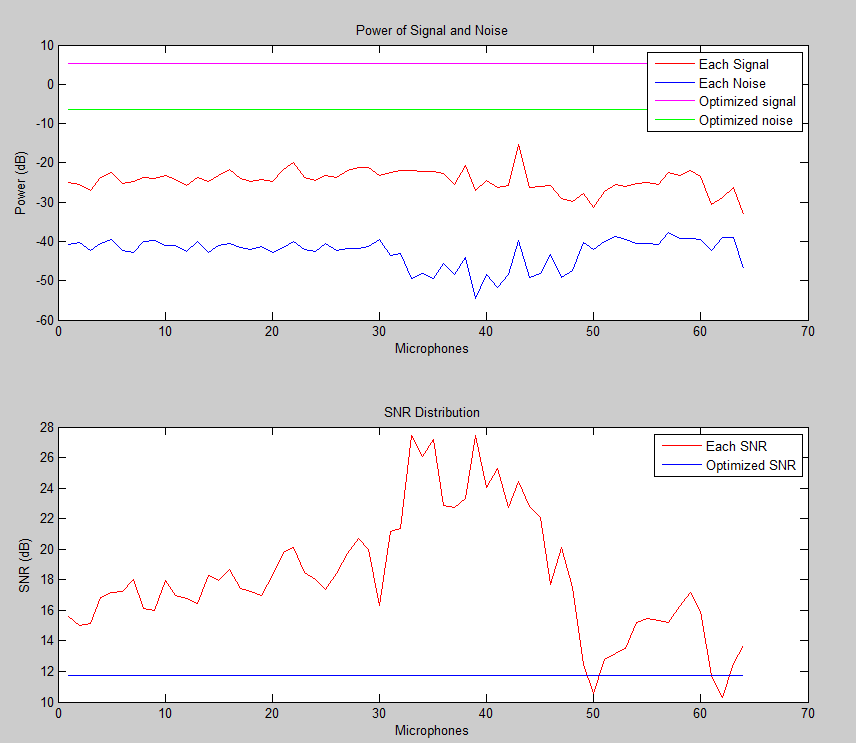
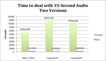
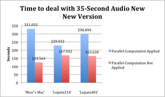
The task for week 3 is to go further to see whether it is possible to speed up the algorithm a little more and make it real-time. As suggested by Mr. Richter Ed to try to connect computers in the same lab as to improve the computation ability, Luting and I made big changes on Matlab code so that finally computers in the same lab could be connected using TCP/IP protocol during week 3. All computers were divided into 2 groups, one manager and several workers. The manager is responsible for distribution of tasks (data) to workers and comparison of the results each worker sends back. The workers equally share the computational loads, relying on the data the manager sends to them. We tested the algorithm, in different labs, to see the optimum number of workers under this distributed-computation-like structure. Not only did we introduce a distributed structure into our simulation, also we managed to lower the computational load for each worker. We deleted a time-consuming function, saving a comparatively large amount of time, and changed the way we timed our algorithm to be more reasonable and precise. By the end of week 3, we eventually make the algorithm real-time, dealing with a 35-second audio file with 30 seconds. Luting Yang went back to China after week 3 and would return one month later. The work afterwards would be on me. After all, this is an independent project. From week 4, the project moved to hardware-related stage. It took a couple of days, in the first place, to fix the microphone array boards. Some of the microphones were out of work due to the microphone itself or bad soldering. Bad soldering on the boards caused ill functioning of amplifier. After the boards worked, Mr. Richter Ed helped me slightly change the Matlab code as well as LabView code and achieved getting the real-time DOA for every second under the distributed-computation-like structure. 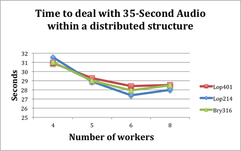 This is my first report for the first 2 weeks of the project. The task assigned by Mr. Richter Ed for these 2 weeks is to optimize the algorithm Luting designed last semester. The former algorithm was created to calculate the direction of arrival (DOA) of sound source based on the data from all 64 microphones, but it took too much time to achieve it. The basic idea of the algorithm to get the DOA in each second is using delay-sum beamforming. However since the original one-second data contain 64*50000 voltage data for all 64 microphones with 50000 samples for each microphone per second, a huge amount of calculation is needed. Luting and I made big progress with the algorithm in the past two weeks. During week 1, we achieved analyzing data in frequency domain. The former version of algorithm did sum in time domain, which means algorithm has to do both fft and ifft, while new version only has to do fft part and roughly double the speed. In addition, we did a lot of adjustments on Matlab code to take the advantage of matrix computation. The benchmark is based on our repetitive tests on computers in different labs. During week 2, we continued modifying the algorithm. A band-pass filter was added into the algorithm before beamforming. The filter magnificently reduced the computation cost, the size of input data reduced from 64*50k to 64*4k, and of course it also greatly speed up the algorithm. Besides, we also modified the Matlab code so that parallel computation, an advanced characteristic of Matlab, could be applied in the simulation. Parallel computation did help and contributed a lot when the computation is much. By the end of week 2, we have been very close to real time, using 36.751s to deal with a 35-second data file. To quantify the improvement, we made a benchmark to see how much faster it is after certain changes happened. The benchmark is based on our repetitive tests on computers in different labs. Thanks for Luting Yang’s voluntary work. He doesn’t satisfy the former performance of his algorithm and wants to challenge himself to make the simulation in Matlab real-time.
|